Tutorial

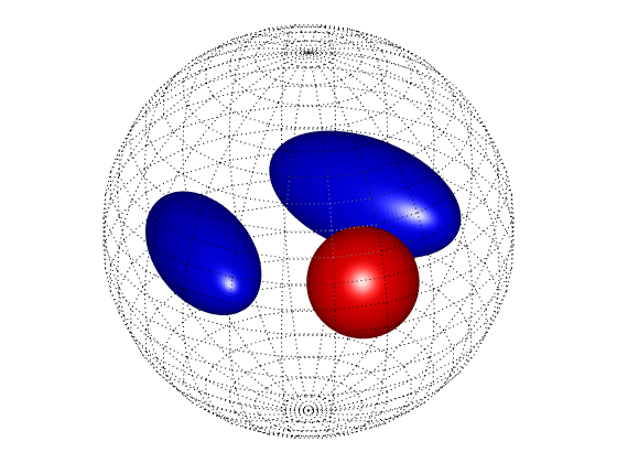
In this tutorial we consider a phantom consisting of conductive inclusions in the unit ball with a known background conductivity.

Inclusion	Center	Radii	Axes	Conductivity
Ball	(-0.09,-0.55,0)	r = 0.273		2
Left spheroid	0.55(-sin(5π/12),cos(5π/12),0)	r1 = 0.468 r2 = 0.234 r3 = 0.234	(cos(5π/12),sin(5π/12),0) (-sin(5π/12),cos(5π/12),0) (0,0,1)	0.5
Right spheroid	0.45(sin(5π/12),cos(5π/12),0)	r1 = 0.546 r2 = 0.273 r3 = 0.273	(cos(5π/12),-sin(5π/12),0) (sin(5π/12),cos(5π/12),0) (0,0,1)	0.5

Forward problem solver

Assuming crEITive has been installed successfully and initialized by run startup we start by defining the needed constants:

% Orientation
rotang=5*pi/12;

% Prolate spheroid on the right
% Center
xr0=sin(rotang)*0.45; yr0=cos(rotang)*0.45; zr0=0;
% Radius
rr=0.42;
% Conductivity
cr=0.5;

% Prolate spheroid on the left
xl0=-sin(rotang)*0.55; yl0=cos(rotang)*0.55; zl0=0;
% Smallest radius 
rl=0.36;
% Conductivity
cl=0.5;

% Axes
A = [cos(rotang),sin(rotang),0;-sin(rotang),cos(rotang),0;0,0,1];

% Ball
% Center
xb0=-0.09; yb0=-0.55; zb0=0;
% Radius
rb=0.21;
% Conductivity
cb=2;

Creating the conductivity objects is then straightforward. Currently crEITive supports two classes of conductivity: piecewise constant and radial. We have to choose the number of quadrature points for each of the inclusions.

% Possible Classes:
        
% Piecewise constant:
%     - PcBallConductivity ( center , radius , amplitude , n )
%     - PcEllipsoidConductivity ( center , radii , axes , amplitude , n )
% Radial:
%     - RadialBallConductivity ( radius , amplitude , innerextent )

% Quadrature points: 2(n+1)² gives the number of quadrature points on
% the unit sphere. The quadrature integrates exactly spherical harmonics
% of degree less than or equal to n. These points are mapped onto the 
% ellipsoid boundary.
n = 10;


% Create different conductivity elements for pcc
SRpc = PcEllipsoidConductivity([xr0,yr0,zr0], ...
                                [1.3*rr, 0.65*rr, 0.65*rr], A', cr, n);
SLpc = PcEllipsoidConductivity([xl0,yl0,zl0], ...
                                [1.3*rl, 0.65*rl, 0.65*rl], A, cl, n);
B1pc = PcBallConductivity([xb0,yb0,zb0], 1.3*rb, cb, n);

% Collect total conductivity data
conddata_pc = MakeConductivityData(SRpc,SLpc,B1pc);

% Plot
PlotPCPhantom(conddata_pc)

To compute the Dirichlet-to-Neumann map of this conductivity distribution we use a function implementing a boundary element method, see Research. For this example we choose the following parameters:

%% Forward map parameters

% Maximal degree of spherical harmonics in the
% computation of the Dirichlet-to-Neumann map.
nd = 10;  

% Mesh used to save the conductivity and q at points.
% Useful to compare the conductivity and reconstruction
% at points of a gmsh mesh.
mesh = 'ball_0p1_3D.msh';  % choose mesh from crEITive/mesh/ folder

savecond = 1;   % {0,1} - save conductivity data or not?
saveq    = 1;   % {0,1} - save q data or not?
parallel = 1;   % {0,1} - parallelize or not? (Requires openMP)

% (optional) Define your own script for running on a cluster
clusterscript = 0; 

% Unique id number for your forward computation
dnmapid  = 1;

The following command then saves all the provided information into a command file in crEITive/commands/dnmap_commands.

% complex  - {0,1} whether phantom is complex or not
% commands - path and name of command file
% log      - path and name of log file

[complex, commands, log] = WritePcCommandsFile(conddata_pc,nd,dnmapid,...
                                               savecond,saveq,mesh);

You may either simply run ./bin/pcc [commands] [log] from your terminal window in the folder crEITive. Or you can provide a script that submits the command to a computing cluster. See submitToDTUCluster.m  for an example; in this case you also provide an email for updates.

% Start
StartDNMAP(method, parallel, complex, commands, log, clusterscript, email)

When the program is done, the resulting Dirichlet-to-Neumann map is saved in the folder crEITive/results/dnmap and is identifiable with the id number.

Reconstruction

Given a Dirichlet-to-Neumann map in the data type described under Data storage we may reconstruct a conductivity using a variety of CGO-based methods (see Research):

% Method used for the reconstruction
%   - calderon for a reconstruction with Calderón approximation.
%   - texp for a reconstruction with texp (Born) approximation.
%   - t0 for a reconstruction with t0 approximation.
%   - t for a reconstruction with full algorithm.
reconmethod = 'texp';

There is a number of reconstruction parameters pertaining to the so-called scattering transform and the regularization of the inverse map

% Computation of inverse Fourier transform
%   - ifft for an Inverse Fast Fourier Transform
ift = 'ifft';

% Resolution of grid where the scattering transform is computed
ngrid = 11;

% Truncation radius (maximum frequency of scattering transform)
% We must have truncrad <= pi*(ngrid-1)^2/(2*ngrid) by Shannon Sampling
truncrad = 9;

% Complex frequency (zeta) size and type.
%   - |zeta| = pkappa*truncrad/sqrt(2) if fixed = 1.
%   - |zeta| = pkappa*|xi|/sqrt(2) for each xi if fixed = 0.
fixed  = 1; % {0,1} choose zeta fixed (1) or proportional (0)
pkappa = 1; % pkappa >= 1

Similar to above we define additional variables and give our reconstruction a unique id.

% Compute conductivity and q on mesh
mesh = 'ball_0p05_3D.msh';  % choose mesh from crEITive/mesh/ folder

dnmapid  = 1; % unique dnmap integer id number of dnmap data
reconid  = 1; % unique reconstruction integer id number
parallel = 1; % {0,1} - parallelize or not?
cluster  = 0;

Computing the inverse map is then straightforward and completely analogous to the forward map

% Commands
[complex, commands, log] = WriteCommandsFile(reconmethod,ift,ngrid,...
                           truncrad,fixed,pkappa,mesh,reconid,dnmapid);

% Start
StartEIT(parallel, complex, commands, log, clusterscript, email);

A number of results is then saved in crEITive/results: conductivity, potential q, scattering transform qhat and trace of CGO solutions, all identified by the reconstruction id. We can make a second reconstruction with the full algorithm:

% Full algorithm
reconmethod = 't';
reconid     = 2;

% Commands
[complex, commands, log] = WriteCommandsFile(reconmethod,ift,ngrid,...
                            truncrad,fixed,pkappa,mesh,reconid,dnmapid);
% Start
StartEIT(parallel, complex, commands, log, clusterscript, email);

Note the results are named with a specific string (conductivity_2_t_nd_10_fixed_ifft_ngrid_11_kap_1_dnmap_1.mat) containing information on the reconstruction parameters.

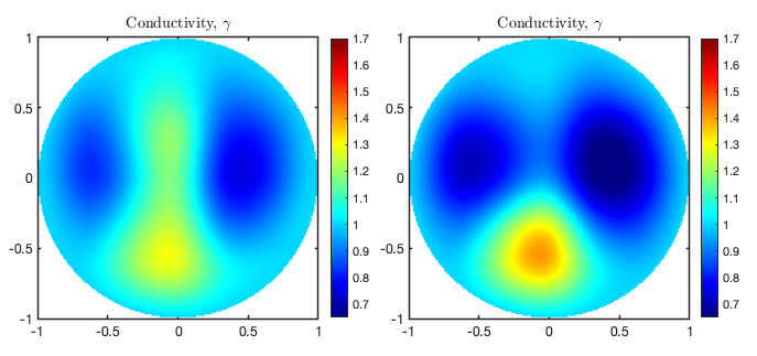
Plots

The results of the reconstruction function allows for simple plots. In this case we compare the reconstructions above corresponding to reconid = 1 and reconid = 2. To make the plots appealing we restrict the plot function to comparing an even amount of results. With Plot2D we may view a 2D slice of our three-dimensional conductivity reconstruction.

% You may choose from {'conductivity','q','qhat'}
type    = 'conductivity'; 

reconid = [1,2]; % reconstruction id
dnmapid = 0;     % include true data by giving dnmapid

v       = [0,0,1];    % normal vector to slice
h       = 0.01;       % stepsize
span    = [0.65,1.7]; % span of type

[ha, pos] = Plot2D(type, reconid, dnmapid, v, h, span);

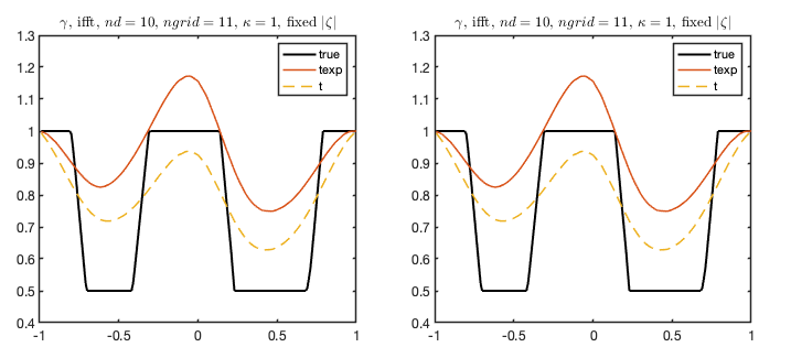
The plot functions returns a figure handle, allowing for simple modification of the figure. Similarly we may want to plot one-dimensional restrictions of results along straight lines. Using Plot1D we can compare several restrictions in subplots.

% You may choose from {'conductivity','q','qhat'}
type         = 'conductivity';

% comp_reconid is a matrix with columns representing 
% plots, in which the elements are ids to types we 
% want to compare in 1D plot
comp_reconid = cat(2,[1;2],[1;2]);

% include true data by giving dnmapids in a vector
include_true = [1,1];

% comp_what is a cell list length == size(comp_reconid,2) 
% of "comparison"-strings. One "comparison"-string in 
% {'method','ift','ngrid','fixed','pkappa'} for each
% column in comp_reconid.
comp_what    = {'reconmethod','reconmethod'};

The columns of comp_reconid corresponds to different subplots and the elements in those vectors consists of the reconstructions we wish to compare. In this example we consider two identical subplots comparing reconstructions reconid = 1 and reconid = 2 with the true phantom.

% Restriction of the conductivity to a line requires a
% direction v and a point center
v            = [1,0,0];
center       = [0,0,0];

h            = 0.01;      % stepsize
span         = [0.4,1.3]; % span of type

[ha, pos] = Plot1D(type,comp_reconid,include_true, ...
                   comp_what,v,center,h,span);

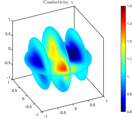
We may also plot several two-dimensional slices of a conductivity distribution in the same plot.

% 3D plots supports only conductivity type of data
reconid = 1; % reconstruction id
dnmapid = 0; % include true data by giving dnmapid

% Slices are given as for the Matlab slice function
xslice  = [-0.6,-0.05,0.6]; % slice vector x
yslice  = [];               % slice vector y
zslice  = 0;                % slice vector z

h       = 0.01;      % stepsize
span    = [0.8,1.4]; % span of type

[ha, pos] = Plot3Dc(reconid, dnmapid, xslice, yslice, ... 
                    zslice, h, span);

Data storage

This document describes how the data are stored in the different results files.

Additional functions

The crEITive software tool includes a number of auxiliary Matlab functions for plotting, reading, writing and computing data:

• plot_piecewise_constant_heart_lungs.m – plots a 3D view of the piecewise constant hearts-lungs phantom used here
• tight_subplot.m – for tight subplots by Pekka Kumpulainen
• read_conductivity.m – reads conductivity.mat files
• read_gmsh_mesh.m – reads gmsh mesh file
• read_q.m
• read_qhat.m
• read_dnmap.m
• snorm.m – computes approximation of L^2-based Sobolev H^s operator norm of matrix approximation of operator
• add_noise_dnmap.m – adds noise to Dirichlet-to-Neumann map according to s-norm
• write_dnmap.m – writes matrix to Dirichlet-to-Neumann map file according to data storage
• gauss_legendre.m – computes nodes and weights for Gauss-Legendre quadrature rule of order n on [-1,1]
• quad_points_unit_sphere.m – computes quadrature points on the unit sphere